1.1   Making Python Tool boxes

A science project (like the one you are going to make), will often contain some repeated and similar sub tasks like loops over different kind of atoms, structures, parameters etc. As an alternative to a plethora of similar Python scripts, made by copy+paste, it is advantageous to put the repeated code into tool boxes.

Python supports such tool boxes (in Python called modules): put any Python code into a file stuff.py then it may be used as tool box in other scripts, using the Python command: from stuff import thing, where thing can be almost anything. When Python sees this line, it runs the file stuff.py (only the first time) and makes thing available. Lets try an example:

• In file stuff.py, put:

  constant = 17
  def function(x):
      return x - 5

• and in file program.py, put:

  from stuff import constant, function
  print 'result =', function(constant)

• Now run the script program.py and watch the output.

You can think of ASE and Dacapo as a big collections of modules, that we use in our scripts.

1.1.1   Fcc Surface Builders

As a non-trivial example of a Python module, we'll try to make a tool box for making fcc surface slabs with arbitrary number of layers. A real fcc surface has a large number of atomic layers, but most surface properties are well reproduced by a slab with just 2 - 20 layers, depending on the material and what properties you are looking for.

The most important cubic surfaces are (100), (110), and (111). For face centered cubic, (111) has most compact atomic arrangement, whereas (110) is most open. Here we'll focus on (111), which is most stable.

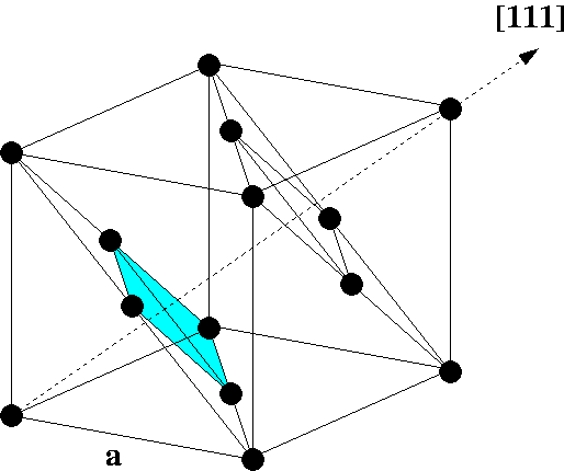
Cubic fcc unit cell

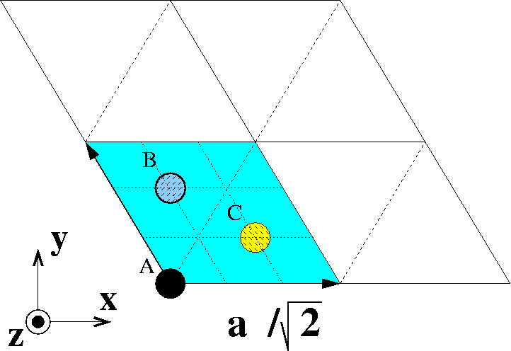
• Find two linear independent vectors that span the primitive surface Bravais lattice of fcc(111). Express vectors in Cartesian coordinates x,y,z in terms of the cubic lattice constant a. Please see figure.

  

  Primitive fcc(111) surface unit cell. Atoms indicate ABCABC... stacking.

• What is the coordination Z (number of nearest neighbors) of an fcc(111) surface atom? What is it for a bulk atom?

• Now that we know the surface geometry, we can setup a toolbox for making surface structures with arbitrary number of layers. Copy the script Build.py to your area. Browse the script and try to understand it. The central part is the function starting with def BCC100(...) that creates a body centered cubic (100) surface.

• Add a function called FCC111 to the Build.py module. This function should build an fcc(111) surface slab. Run the script until you are sure that your new function works (by running the script, you activate the self test in the last few lines of the script, starting at if __name__ == '__main__': - the self test is not done, when you import from your module, though).

hint:

Square roots are calculated like this: 2**0.5 or sqrt(2) (the sqrt function must first be imported: from math import sqrt).

Note

>>> 1 / 3
0
>>> 1 / 3.0
0.33333333333333331

1.2   Aluminum fcc(111) Surface Slabs

In this section, we'll study how surface properties converge, as the slab becomes thicker and thicker.

1.3   Adsorption of H on the Al(111) surface

One of the most prominent applications of density functional theory is making predictions about alternative atomic structures, when adsorbates are present on the surface. In this exercise, we study the adsorption of H onto Al(111). For simplicity, we use a small and thin Al(111) slab: A 1 x 1 surface unit cell of a two layer Al(111) aurface and deposit a monolayer of H onto the Al(111) slab. The thermodynamics of the H/Al(111) system is governed by the adsorption potential energy surface (PES), i.e. the energy of H/Al(111) as function of the H atom coordinates; in this section, we try to map out and understand the adsorption PES.

• Why are high symmetric sites on the Al(111) surface good candidates for stable adsorption sites?
• How many inequivalent high symmetry adsorption sites are present on a two layer Al(111) 1 x 1 surface unit cell. What is the coordination Z (i.e. number of nearest Aluminum neighbors of an H atom) in each adsorption site?
• There are two inequivalent hollow sites. What is the difference?
• We'll adsorb a monolayer of H in all high symmetry sites of the Al(111), i.e. one H atom per Al(111) 1 x 1 surface unit cell.
  • Use a unit cell with a height of 10.0 Å.
  • We relax ionic positions. For simplicity, we'll freeze the Aluminum slab atoms, and only relax the H adsorbate. This is done in the script Relax.py.

• If you want the relaxation to converge quickly, it is necessary to make a qualified guess on the equilibrium position of the H adsorbate. A simple way is to assume that equilibrium bond lengths are the sum of the respective covalent radii. In our case r_Al = 1.18 Å and r_H = 0.37 Å. You may get these kinds of data at http://www.webelements.com. Select the initial adsorbate elevation over the surface for each adsorption site, so that Al-H bond lengths are 1.55 Å.

• Run your script and calculate the total energies of the different adsorption sites, thereby determining their relative energetic stability.

• Suppose now that an H atom diffuses from one hollow to a neighboring hollow site at the surface. What is the activation energy for this process? Assuming a prefactor of 10¹³/sec, how many times does the diffusion take place at T = 100 K, 200 K, 300 K and 500 K.

• For biological catalytic processes, a popular rule of thumb is that the rate doubles for every temperature increase of 10 K around room temperature? What activation energy does this correspond to?

• If one would want to investigate the diffusion process properly, how would you do this? What would have to be changed from the present setup?

• Look at the relaxed configurations with the plottrajectory command:

  plottrajectory ontop.nc

• Repeat one of your H/Al(111) calculations with slightly more vacuum and use the keyword dipole=True when you create the Dacapo calculator. This will add a dipole layer in the middle of the vacuum region. In order to understand what is going on, take a look at the electrostatic potential and the Fermi-level, when the calculation has finished:

  >>> from Dacapo import Dacapo
  >>> atoms = Dacapo.ReadAtoms('out.nc')
  >>> calc = atoms.GetCalculator()
  >>> print calc.GetFermilevel()
  >>> v = calc.GetElectrostaticPotential()
  >>> nx, ny, nz = v.shape
  >>> print nx, ny, nz
  >>> import Numeric as num
  >>> vz = num.sum(num.sum(v)) / (nx * ny)
  >>> import Gnuplot as gp
  >>> plot = gp.Gnuplot()
  >>> plot.plot(gp.Data(vz, with='lines'))
  

  The workfunction of a surface is defined as the energy required for an electron to escape from the surface. What are the workfunctions of the two surfaces?

1.4   Making nice plots with VMD

One functionality in ASE is that you can make nice plots of the atomic configurations, the Kohn-Sham wave functions and the electron density. Apart from that these plots can be made to look very nice, they can also visualize things which otherwise are hard to analyze or explain. ASE supports visualization tools like VTK, Rasmol and VMD. We will focus on VMD.