Examples
or how-to's
Contents
- 1 CO molecule
- 2 Relaxing the CO molecule
- 3 Al Equation of State
- 4 H/Co(1000)
- 5 Using filters and dynamics
- 6 h2o dissociation
- 7 VTK plotting
- 8 Calculating a band diagram
- 9 Nudged Elastic Band
- 10 Vibrational Calculation
- 11 Dipole correction and electrostatic potential
- 12 STM images - Al(100)
- 13 Localized Wannier orbitals
- 14 Transport calculations
- 15 Bayesian Error estimation in Density Functional Theory
1 CO molecule
Setting up a CO molecule in a box. This is the minimum script (or close to the mimimum) one can define:
CO_in_a_box.py
2 Relaxing the CO molecule
This is the second minimum script one could define. This relaxes the CO geometry until the magnitude of the force on each atom is less than 0.05.
CO_relaxed_in_a_box
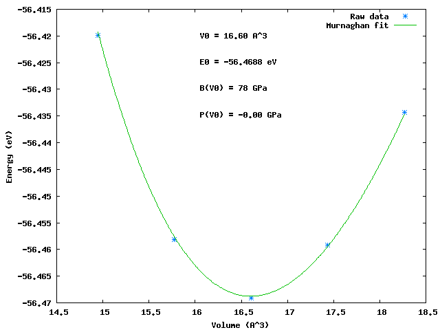
3 Al Equation of State
This example uses the EquationOfState Module and GeometricTransforms Module to find the ground state lattice constant and bulk modulus of bulk Al in the fcc crystal structure.
Al_equation_of_state
Once the jobs are done, you could run the command line utility eos to view the results again and save the figure as a png file.:
eos -m -s Al_murn.png bulkAl_*.nc
eos takes many options:
eos [-m -b --bm -a -t -v -p --all -q -s [filename]] [ncfiles]'

these flags specify the equation of state to use. Several can
be selected at a time

-m   'Murnaghan',
-b   'Birch',
--bm 'BirchMurnaghan',
-t   'Taylor',
-p   'PourierTarantola',
-v   'Vinet',
-a   'AntonSchmidt'
--all runs all equations of state

-s  filename  saves figure in file, format by extension. png and eps supported.
-q  quiet, no gnuplot window

if no ncfiles are provided, it uses all ncfiles found in the
current directory. shell patterns like bulk*.nc are allowed to
use only files matching that pattern.
Typical results look like:
Murnaghan: PRB 28, 5480 (1983)
V0(A^3)       B(Gpa)   E0 (eV)    pressure(GPa)
 16.60        78.27     -56.4688       -0.00
chisq = 0.0000
lattice constant = 4.05 angstroms
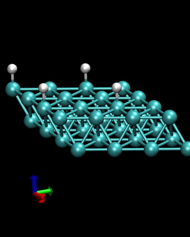
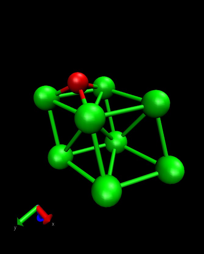
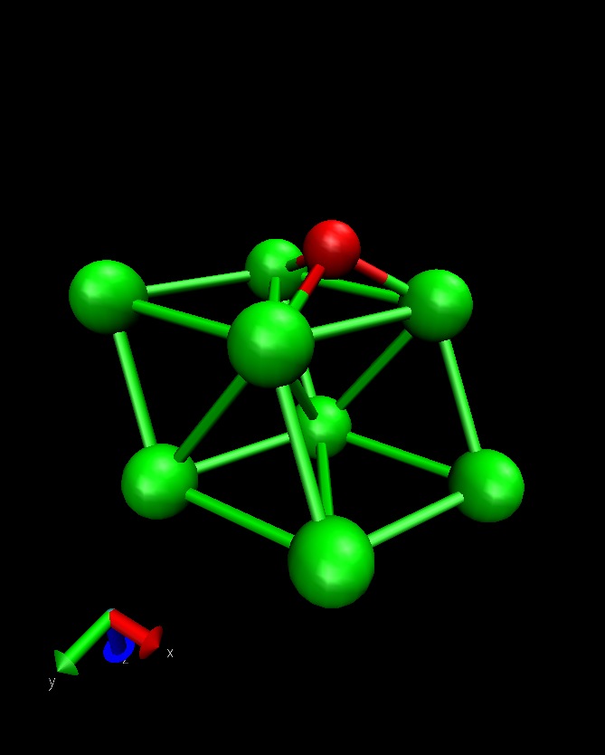
4 H/Co(1000)
This example calculates the total energy of a Hydrogen atom on a Co(1000) surface:
H_Co_ontop
This is how the surface looks like, using:
>>> from ASE.Visualization.RasMol import RasMol
>>> RasMol(slab, (2,2,1))
5 Using filters and dynamics
The CO molecule is relaxed using a constrain filter Subset and the MDMin dynamics:
filter
A NetCDF trajectory is added to the dynamics, writing to a file CO-trajectory.nc.
The minimization path can be viewed after the run using the tool plottrajectory from the ASE/Tools directory:
plottrajectory Co-trajectory.py
6 h2o dissociation
This example use the Subset filter together with the FixBondLenght filter to find the barrier for dissociating the h2o molecule:
h2o-quasi-Newton
The script use the quasi-Newton algorithm, reusing the Hessian matrix from one bond length to the next. This can speed up the convergence significantly. The plot below shows the energy versus the total number of iterations, ie. for all bond lengths, comparing different minimization algorithms:
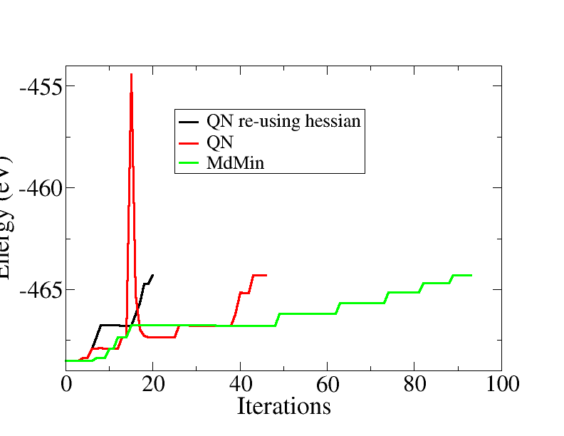
The total number of iteration is reduced from 95 for MDMin, to 45 for the quasi-Newton and finally to 20 for the quasi-Newton, re-using the Hessian from the previous bond length.
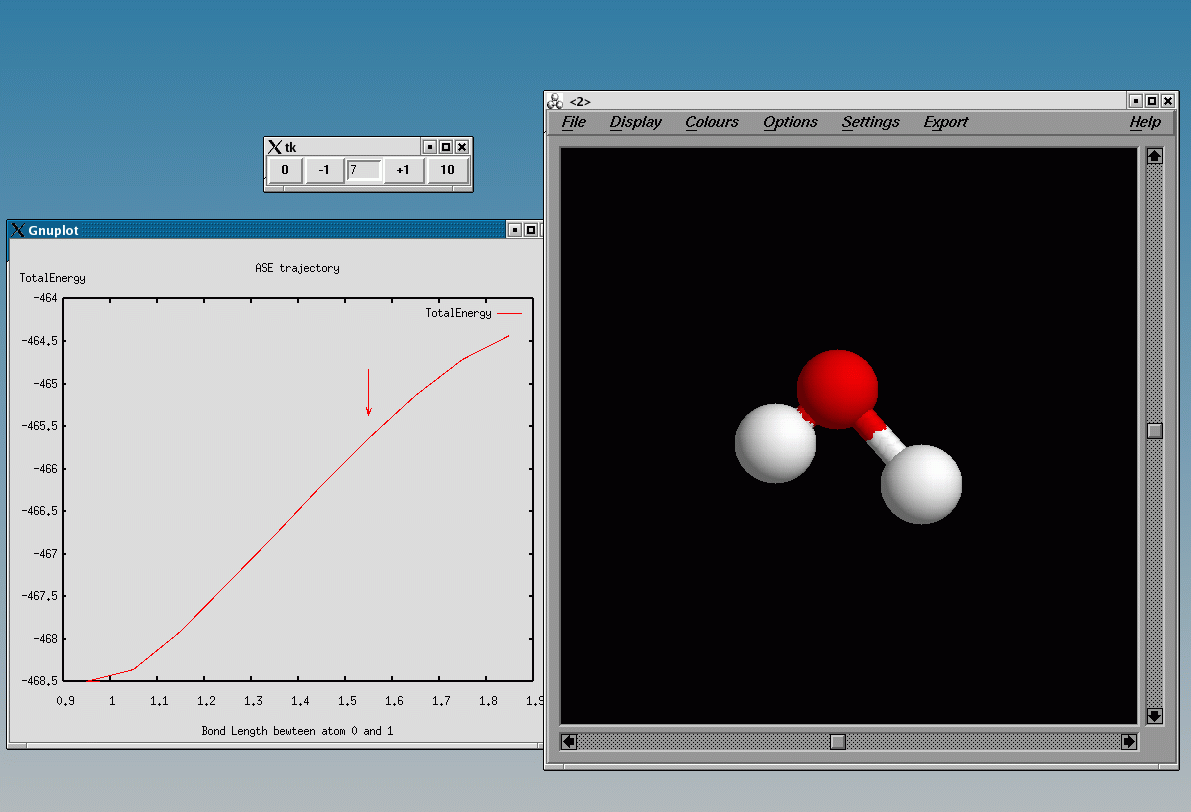
Using the plottrajectory tool one can plot the constrained bond length against the total energy:
plottrajectory.py -p [[BondLength(0,1),TotalEnergy]] h2o-dissociation.nc
This will look like:
7 VTK plotting
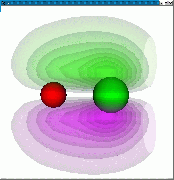
This example illustrates how one can use VTK to make a combined plot of the wavefunction of a CO molecule, together with the molecule itself:
plotwave1
Run the example like:
python -i plotwavefunction.py <band number>
This example also illustrates how a calculation can be restarted from a existing dacapo NetCDF file.
Using:
python -i plotwavefunction.py 3:
the following plot is produced:
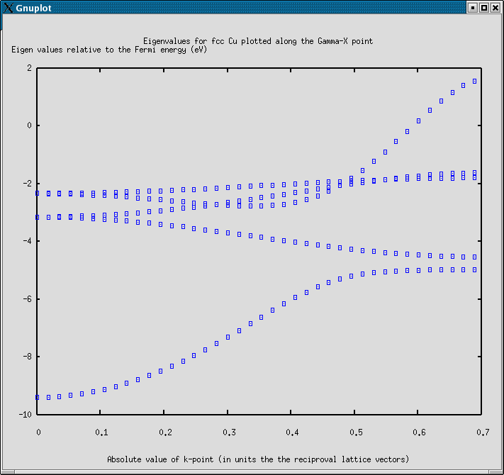
8 Calculating a band diagram
The example shows how the band diagram between the Gamma point and the X point in the Brillouin zone can be calculated for Cu in a fcc lattice.
The plot produced by this example is just plotting the individual eigenvalues, not making a real bandstructure plot.
In order to do a band structure calculation one can proceed as follows:
- First do a calculation with a usual k point sampling.
- From this calculation get the self-consistent electron density and use this density as input to the band diagram calculation.
- Do the band structure calculation non-self-consistently, i.e. a Harris calculation where the electron density is not updated.
Note that the Fermi levels for the two calculations may differ (by a significant amount !!). In general the Fermi energy from the original calculation should be used.
harris
The resulting plot looks like:
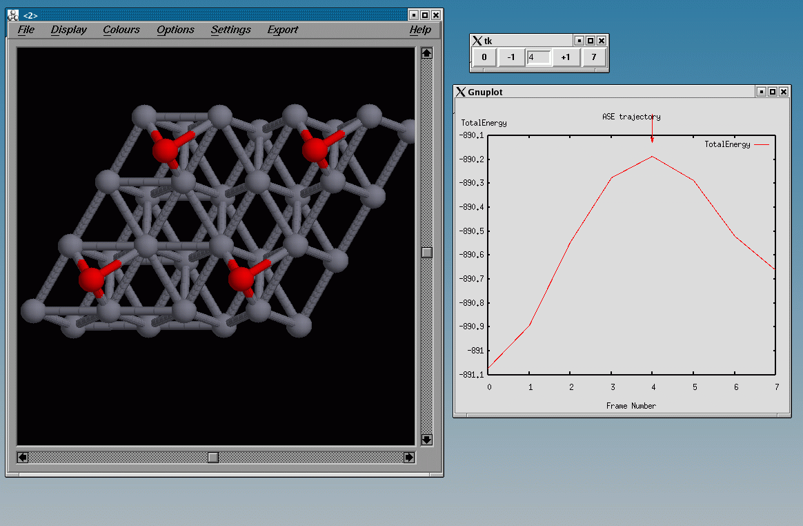
9 Nudged Elastic Band
The Nudged Elastic Band method is a technique for finding transition paths (and corresponding energy barriers) between given initial and final states. The method constructs a chain of "images" of the system. See the ASE NudgedElasticBand filter for more details.
To illustrate this functionality, we will consider O diffusion on Al(111) between an fcc and hcp hollow site. This example use the quasi-Newton algorithm for minimizing the band. See also Mimimizing the Nudged Elastic Band for a general description of this method:
neb
The initial and final state looks like
After the run a set of dacapo files out.*.nc are produced and a set of trajectory files image*.nc, one for each image. Each of these files will contain the number of timesteps done by the quasi-Newton algorithm. You can check the overall convergence from the quasi-Newton log file:
> grep QN qn.log
  QN: energy maxforce -8013.409959 2.705231
  QN: energy maxforce -8014.081961 0.704026
  QN: energy maxforce -8014.149499 0.152324
  QN: energy maxforce -8014.151499 0.042264
In this case the minimization is done in 4 steps, each steps involves calculating the energy and force for each image.
A restart script can look like this:
restart-neb
This script reuse the Hessian matrix written (by default) to the file hessian.pickle. restart-neb.py write to the log file qn-restart.log:
> grep QN restart.log
  QN: energy maxforce -8014.151534 0.042264
Running the restart-neb.py script should not involve doing any new calculations, because the band has allready been converged in the neb.py script.
At the end of neb.py and neb-restart.py the last timestep for each image are put in a new trajectory file neb-path.nc. Instead of a timeseries this trajectory contains the M images for the converged path.
(This last step will probably be added to ASE.Utilities)
The result of:
plottrajectory neb-path.nc
should look like this, showing the point close to the transition state:
10 Vibrational Calculation
You can calculate the vibrational modes of a ListOfAtoms in the harmonic approximation using the ASE.Utilities.VibrationalCalculation module. The ListOfAtoms should either be in a ground state (i.e. fully relaxed) or at a saddle point (i.e. a transition state, as calculated by NEB). You can select a subset of the ListOfAtoms for which to find the vibrational modes, specify the displacements for each atom, and whether forward, backward or centered finite differences are used to calculate the Hessian matrix. The module calculates vibrational frequencies, zero-point energy and the vibrational eigenmodes of the system you specify. The module should be calculator independent, but it does rely on the calculator having a ReadAtoms method, and it uses netcdf files to get data from.
Note: problems with running vibrational calculations in dacaop were reported https://listserv.fysik.dtu.dk/pipermail/campos/2008-May/002430.html, and running dacapo in StayAlive (https://wiki.fysik.dtu.dk/dacapo/Manual?highlight=%28StayAlive%29#dacapo-fortran-program-python-interface-communication) mode turned out to be a workaround.
You must run the CO_relaxed_in_a_box.py script above before you can calculate the vibrational frequencies of CO.
CO_vibrations
The output of this script looks like this:
2124 1/cm
Imaginary frequency
Imaginary frequency
4 1/cm
398 1/cm
401 1/cm
Zero-point energy = 0.18 eV
The main experimental vibrational frequency for CO is 2180 1/cm. Note the calculation produces 6 frequencies, while for CO we expect only one (3N-5 because its linear). The module calculates 6 modes, but 3 of them are translational; these modes should have frequencies of 0, and correspond to the 3 smallest (including the imaginary ones, which likely had small, but negative eigenvalues. There are also 3 rotational modes for molecules (only 2 for linear molecules). The other 2 modes correspond to the rotational modes, and the magnitude of them suggests that the box is not big enough (in other words, the CO molecules are close enough to interact). Try this set of calculations in a bigger box, you will see it makes a difference.
On slabs it can be a little different. If you only look at the modes of an adsorbate, then depending on the potential energy surface, the three translational modes can be converted to three frustrated translations, and likewise with the three rotational modes. So an adsorbate could have up to 3N vibrational modes.
You should read the source file in detail to see all the options and things that can be done with it. You can find it in ASE/Utilities/VibrationalCalculation.py
11 Dipole correction and electrostatic potential
Using the method calc.DipoleCorrection() or the keyword dipole you can activates the interslab dipole electrostatic decoupling. Presently, this feature is only active along the third unit cell vector so you need to choose unit cell accordingly. Corrections for higher electrostatic multipoles are not implemented presently. This correction is calculated for a O atom on a Al(111) surface in the example:
electrostatic
You can get information on the dipole correction by using:
grep DIP Al111-O.out
This will give the output:
DIP:   u_damp       u    Field_1  Field_2  Work_f1  Work_f2  V_jump   E_dip
DIP:     [eA]     [eA]    [V/A]    [V/A]     [eV]     [eV]     [V]     [eV]
DIP:     0.000    0.142      -        -        -        -      0.000    0.000
..
DIP:     0.338    0.339    0.000    0.000    4.178    6.331    2.155    3.256
DIP:     0.338    0.338    0.000    0.000    4.178    6.332    2.155    3.256
electrostatic.py plots the electrostatic potential:
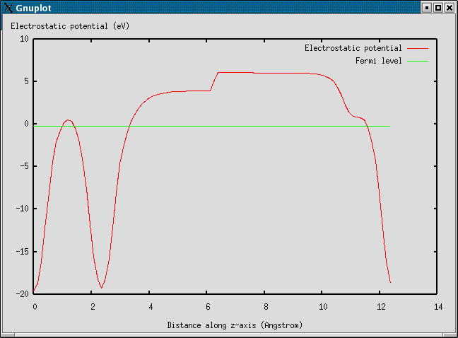
For more details see the workfunction document
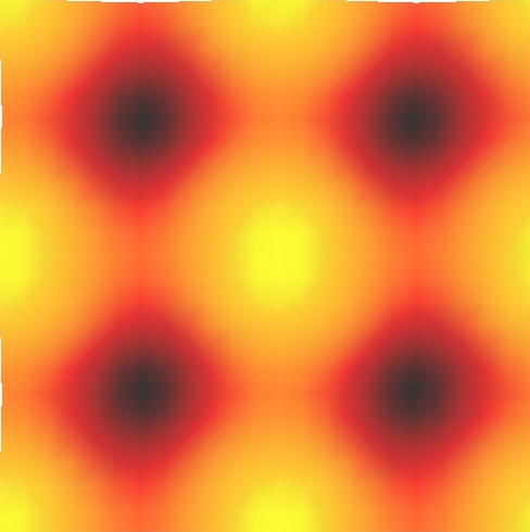
12 STM images - Al(100)
This example use the ASE STMTool class to make a STM images of a Al(100) surface:
STM.py
For more details see the STM tutorial.
The resulting image is shown below:
13 Localized Wannier orbitals
Below are examples of using the ASE Wannier class.
This examples shows how to construct Wannier functions for an ethylene molecule (C2H4):
Wannier-ethylene
This example shows how to construct Wannier functions for a linear chain of 4 Pt with periodic boundary conditions. The gamma-point approximation is applied:
Wannier-Pt4
This example shows how to construct Wannier functions for an infinite,linear chain of Pt atoms. The Wannier functions are constructed using k-points:
Wannier-Ptwire
This example shows how to construct Wannier functions for iron-bcc. Wannier functions are constructed for spin up and spin down states separately:
Wannier-Fe-bcc
For more details see the Wannier tutorial.
14 Transport calculations
This example illustrates the use of the transport module by application to a simple 1d tight-binding model:
transport_1dmodel
For more details see the Transport tutorial.
This example shows how to construct a Wannier function Hamiltonian matrix to be used for a subsequent transport calculation:
setupham
For more details see the Transport tutorial.
15 Bayesian Error estimation in Density Functional Theory
Two examples of error estimation using ensembles are given below. For more details see the GPAW Ensemble Tutorial.
Error estimation of the binding energy of the H2 molecule:
bee
Error estimation of the bond distance and frequency of the H2 molecule:
bee2